ORCID 0000-0001-6232-9096 · daniel@activeinference.institute
DOI 10.5281/zenodo.23676081 · GitHub v0.5.0
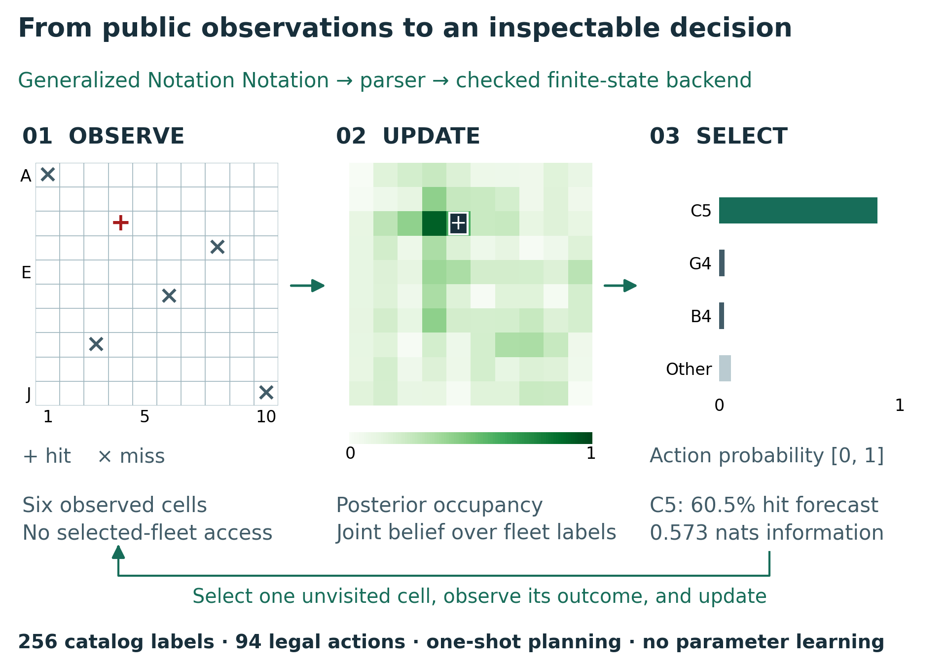
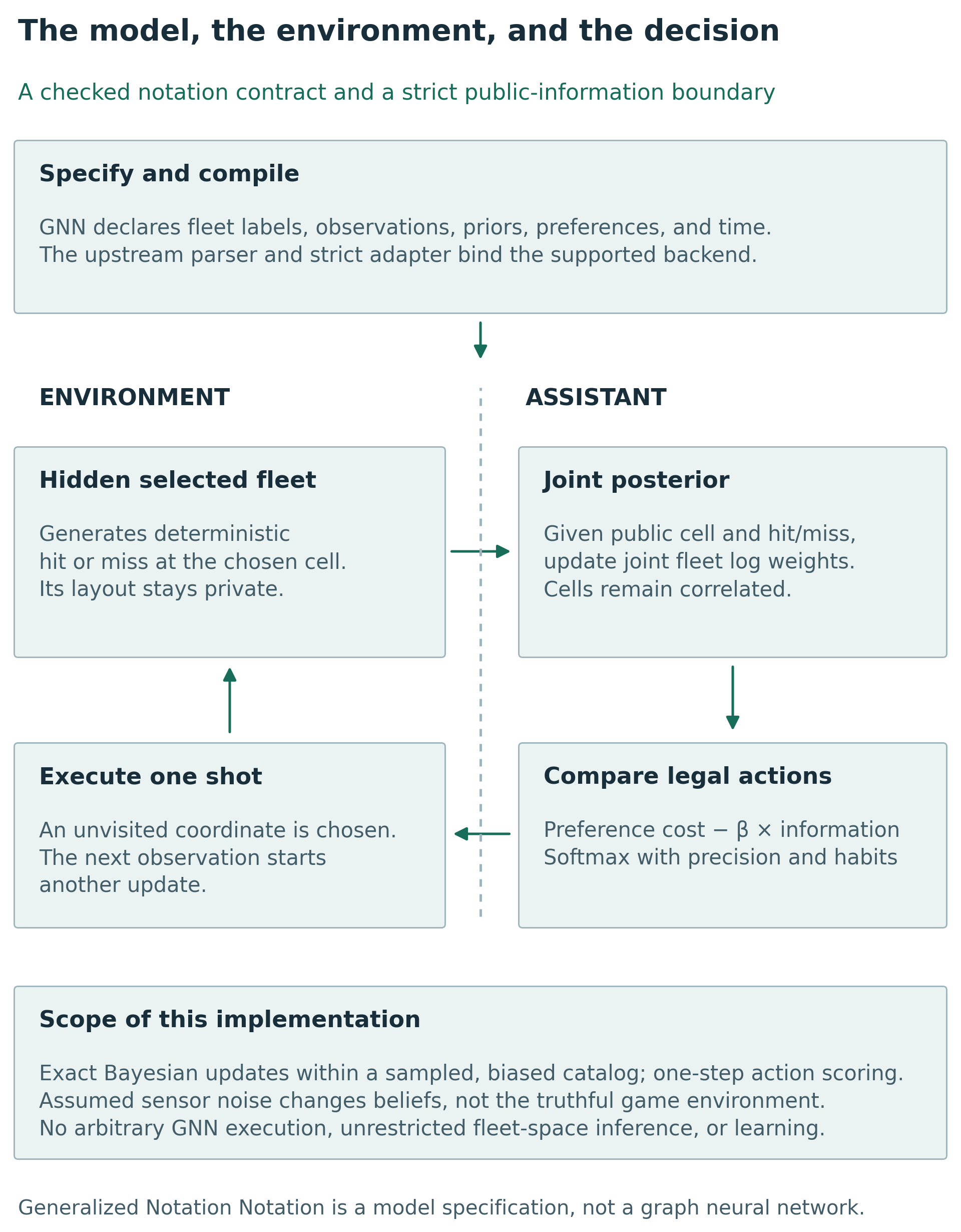
Version 0.5.0 from the Active Inference Institute. The graphical overview introduces the model and interface. It does not claim unrestricted Battleship inference, multi-step planning, parameter learning, or measured educational benefit.
From GNN to a decision
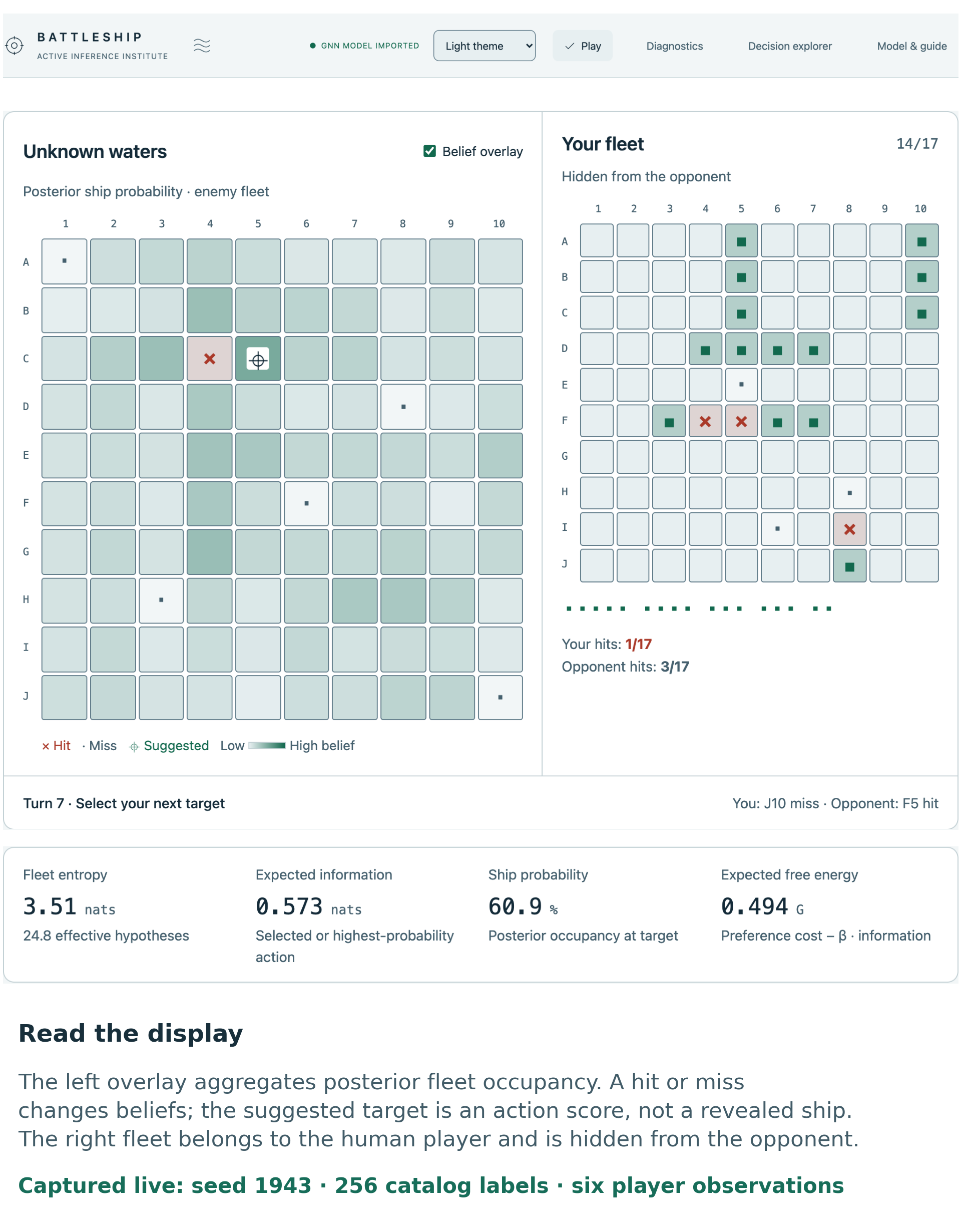
Play and inspect beliefs
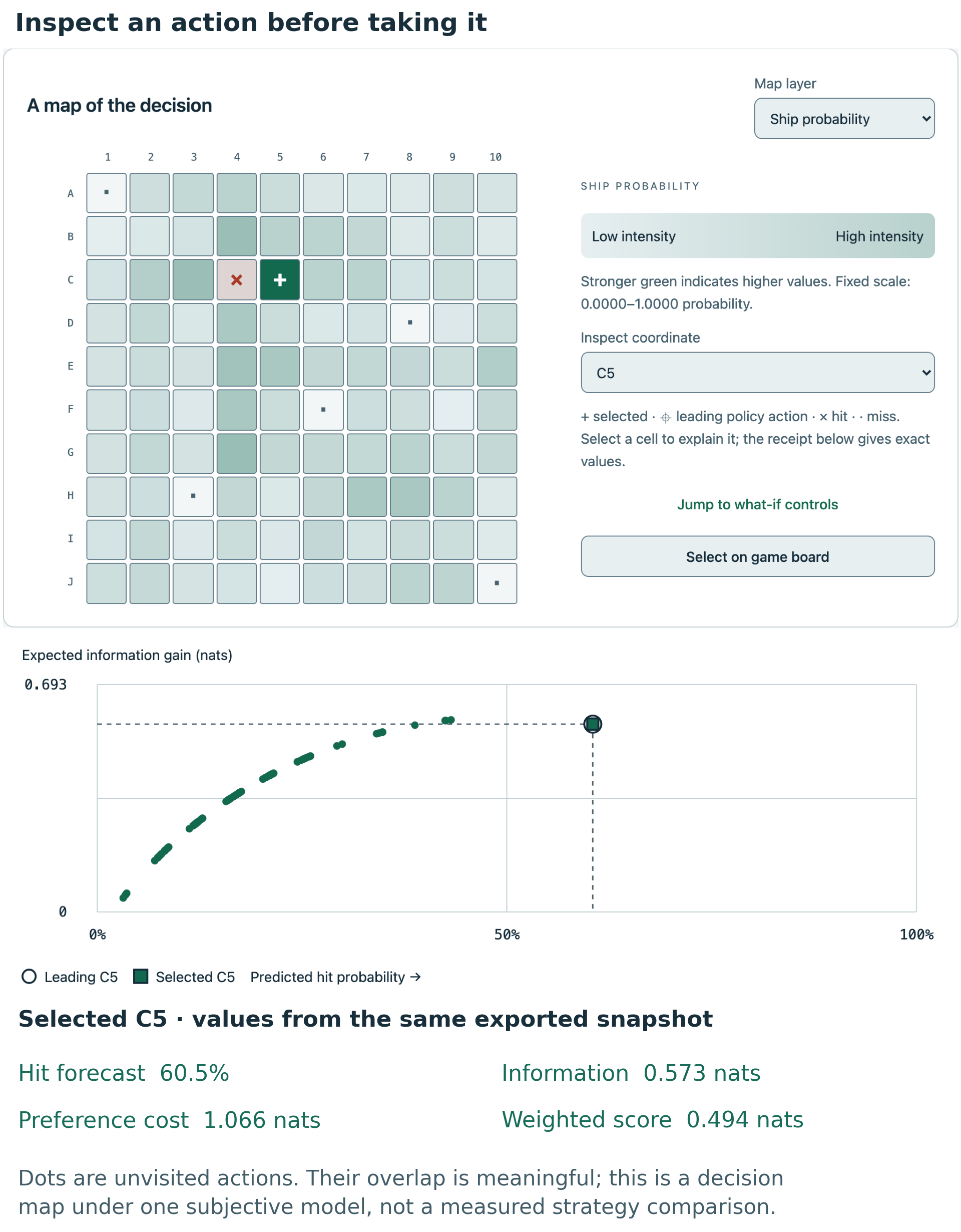
Explain the next action
Abstract
Active inference models connect beliefs, preferred outcomes, and information-seeking actions, but an implementation can obscure the assumptions behind its displayed quantities. We present a browser-based Battleship dashboard whose executable contract begins with a Generalized Notation Notation (GNN) specification. The assistant performs exact categorical Bayesian inference conditional on a reproducibly sampled finite catalog of legal fleets, and evaluates a one-step preference-and-information objective. An interactive decision explorer exposes occupancy, observation forecasts, information gain, preference cost, action probabilities, hypothetical posteriors, and parameter sensitivity for either actor. The selected fleet remains outside the assistant’s information boundary. We derive the implemented quantities, distinguish expected from realized information, and connect the model to active learning, active search, partially observable planning, and prior Battleship research. A two-fleet example isolates the preference–information trade-off. A retained descriptive demonstration motivates a prospectively specified 1,280-search follow-up across 256 fresh paired catalog/truth units and five strategies. Completion shots, five-shot hits, and normalized label entropy receive 24 planned Holm-adjusted paired sign tests, alongside descriptive paired mean-effect intervals. Standard greedy EFE and pragmatic completion counts tie in every pair. Pure epistemic selection has less favorable completion sign balance in both size strata. At 4096 labels, information weighting has favorable five-shot label-uncertainty sign balance; its completion comparison is not rejected. These findings concern the declared generator and objectives, not a generally superior strategy. Seeded traces, source hashes, tests, and a three-edition manuscript build support inspection and reuse. The contribution is an explicit, composable implementation and its interpretable evidence, rather than a new inference principle, an unrestricted Battleship solver, or a validated educational intervention.
A typed core package and headless replay-analysis commands support reuse outside the browser. The Active Inference Institute publishes version 0.5.0 with source and reproducibility materials at the Institute’s public Battleship repository and the manuscript archived on Zenodo, DOI 10.5281/zenodo.23676081. The tagged GitHub release distributes the manuscript, interactive reader, dashboard, reusable core package, and a captioned 20-minute explanatory video with slides and transcript.
Keywords: active inference; Bayesian active sensing; expected information gain; Battleship; Generalized Notation Notation; reproducible software.
1 Battleship as a model of active sensing
Battleship offers a concrete setting for inspecting the relationship between finding a target and learning where targets might be. A shot returns a small observation, yet constrains a correlated collection of possible fleets. A cell with high occupancy probability can be attractive because it is likely to yield a hit. A cell with intermediate probability can be attractive because its possible outcomes distinguish hypotheses. Those objectives need not select the same action, and neither immediate criterion by itself solves a multi-step search problem.
Discrete active inference provides a useful language for making these
choices explicit: hidden states, observation likelihoods, prior beliefs,
outcome preferences, and policy distributions (Friston et al.
2017; Da
Costa et al. 2020). Its epistemic and pragmatic action values
motivate the decomposition displayed here (Friston et al. 2015). Existing practical
resources already support model construction and discrete-state
implementation, including a step-by-step tutorial and the
pymdp library (Smith et al.
2022; Heins et
al. 2022). The present dashboard complements that work with a
small browser implementation in which a reader can connect a spatial
decision to numerical inputs, hypothetical outcomes, and an exported
record. Whether this improves learning is a question for a future
educational study.
We distinguish the environment that generates shot outcomes from the assistant’s subjective generative model. The likelihood’s noise setting describes the assistant’s assumptions, while the environment returns deterministic occupancy. This uses discrete active-inference vocabulary without implementing neuronal process dynamics or learning model parameters (Friston et al. 2017; Smith et al. 2022).
The contribution has three parts. First, a source-identifiable GNN specification is imported through the actual upstream parser and constrained by a strict executable adapter. Second, separate game, inference, analysis, session, and interface modules expose a complete inspectable path from public observations to actions. Third, reproducible examples and a scholarly manuscript explain the implemented mathematics and its limits. The paper does not claim priority for Bayesian Battleship search, information gain, or the integration of epistemic and pragmatic action values.
1.1 Prior work on information gathering and target search
Information-based query selection predates this application. MacKay emphasizes that an acquisition objective depends on the information sought and the assumed hypothesis space (MacKay 1992). Bayesian active learning expresses expected posterior entropy reduction as predictive entropy minus expected conditional entropy (Houlsby et al. 2011). Shannon’s discrete entropy supplies the units and mathematical vocabulary (Shannon 1948). Here the target of inference is a finite latent fleet label, rather than a Gaussian-process parameter, a neural network, or a learned likelihood.
Active search asks a different question from generic uncertainty reduction: how should observations be chosen to discover targets under a task-specific utility? Garnett and colleagues formalize that distinction and show why planning horizon matters (Garnett et al. 2012). Likewise, a partially observable Markov decision process (POMDP) can value information through its consequences for later reward; information gathering is not absent from conventional reward-based planning (Kaelbling et al. 1998). Our one-shot score is an interpretable restriction, not an alternative proof of optimal planning.
1.1.1 Human search and question asking in Battleship tasks
Battleship-related research includes several distinct problems: choosing where to look, constructing questions about a hidden arrangement, and planning actions whose value depends on later observations. Human spatial-search studies provide especially relevant precedent. Gureckis and Markant studied a 10×10 task in which participants uncovered cells to identify three hidden colored rectangles and subsequently reconstructed the arrangement (Gureckis and Markant 2009). Their Bayesian observer valued observations through expected savings under sampling and reconstruction costs. Although visually similar to Battleship, this task revealed rectangle identity rather than binary occupancy, and success concerned recovering the arrangement rather than hitting every ship segment. It therefore supplies a precedent for model-based information search, rather than a benchmark directly interchangeable with the present game.
The distinction between learning and task utility also appears within this experimental lineage. Markant and Gureckis compared expected information gain with expected savings, including a modified search task using letter-shaped targets (Markant and Gureckis 2012). Their subsequent work separated uncertainty about the next feedback label from information gained about the hidden configuration by introducing unreliable observations near adjacent shapes (Markant and Gureckis 2014). These distinctions matter when interpreting our information display. Under the dashboard’s stated likelihood, conditional observation entropy is constant across candidate actions, so information gain and predictive binary entropy rank cells identically. This algebraic equivalence does not establish which calculation a person uses, and the dashboard’s subjective noise setting does not reproduce the location-dependent interference manipulation.
A separate line of work expands the query space beyond individual cells. Rothe, Lake, and Gureckis represented questions as programs that return answers when evaluated on possible worlds, combining informativeness with complexity and answer-type features (Rothe et al. 2017). Their task used three colored ships of variable length on a 6×6 board. Participants could ask questions with single-word answers about properties such as size or spatial relations. This is a substantially richer action space than firing at one coordinate. A question can distinguish many configurations without identifying the occupancy of any particular targeted cell, and its answer need not be binary. Their program model consequently addresses the construction of queries as well as their evaluation.
Related experiments distinguish generating a question from recognizing a useful one. Rothe and colleagues compared freely produced questions with rankings of supplied questions using Bayesian measures of question quality (Rothe et al. 2018). They later extended the analysis to goals that concern particular properties of a board and to question evaluation after an earlier answer (Rothe et al. 2019). The latter experiments asked participants to rank supplied candidates; they should not be described as unrestricted sequential gameplay. Grand and colleagues subsequently combined language-based question proposals, translation into executable programs, and expected-information evaluation in the single-turn Battleship question task (Grand et al. 2024). Together, these studies motivate explicit attention to the hypothesis space, query language, answer model, and task objective. They do not establish educational efficacy or strategy superiority for this application.
Crombez and colleagues analyze a different Battleship problem after a first hit: a single known shape is translated on an infinite lattice, and an adaptive binary decision tree minimizes worst-case misses (Crombez et al. 2020). Its cost is not simply the tree height. That result concerns neither full-fleet catalog search nor the five selectors tested here; it clarifies why observations, planning horizon, and stopping objective must be matched before comparing strategies.
Other precedents further delimit the comparison. Silver and Veness evaluated Monte Carlo planning in a single-agent Battleship search environment with different placement constraints and a long-run objective (Silver and Veness 2010). Grand and colleagues’ collaborative question-and-shot paradigm combines actions absent from the present interface (Grand et al. 2026). Even physical Battleship rules require qualification: the inspected Hasbro A3264 sheet matches the five ship lengths but identifies the ship on a hit, whereas our inference input retains only hit or miss (Hasbro 2016). Finally, Sevenster’s complexity result concerns the solitaire layout puzzle, not this fixed-size shot-selection model (Sevenster 2004). Our contribution is an inspectable finite-catalog implementation with explicitly bounded observations and one-step valuations. It is not a new general theory of Bayesian Battleship, a question-generating agent, or a proof of optimal play.
1.1.2 The meaning of expected free energy
Expected free energy (EFE) also requires careful terminology. Technical treatments distinguish it from simply projecting variational free energy into the future (Millidge et al. 2021). Parr and Friston’s named generalized free energy formulation is a different construction (Parr and Friston 2019). The dashboard’s phrase “generalized EFE” denotes only its explicitly defined information-weighted score. We use “weighted one-step objective” when discussing that extension, without identifying it with the named generalized-free-energy formulation.
2 Finite fleet beliefs and one step action selection
Definitions fix the assumed distributions and objective; propositions state identities under those assumptions. The posterior update appears in eq. 3, the action policy in eq. 6, and the realized surprise identity in eq. 9. These labels and formalism numbers are generated consistently across editions.
2.1 Hidden fleet labels and public observations
Definition 1 (Finite fleet model). Let \(S=\{1,\ldots,M\}\) index a catalog of complete legal fleets on an \(N\times N\) board. Let \(x(s,a)\in\{0,1\}\) indicate occupancy of cell \(a\) in entry \(s\). Ships are straight, do not overlap, and may touch. The default model has \(N=10\), ship lengths \((5,4,3,3,2)\), and \(M=4096\). A seeded bounded randomized placement procedure constructs the catalog; it is not a uniform sampler over the space of all legal fleets. The environment draws a label uniformly from that same catalog. Duplicate entries retain their multiplicity and prior mass.
The state is static. A shot queries one previously unvisited cell and returns \(o\in\{0,1\}\), denoting miss or hit. The assistant’s subjective likelihood and prior are
\[A(1\mid s,a)=\epsilon+(1-2\epsilon)x(s,a),\qquad A(0\mid s,a)=1-A(1\mid s,a),\qquad{(1)}\]
\[B(s'\mid s)=\mathbf{1}[s'=s],\qquad D(s)=M^{-1}.\qquad{(2)}\]
The permitted likelihood parameter is \(0\leq\epsilon\leq0.25\). Actual game feedback always equals selected-fleet occupancy. Thus positive \(\epsilon\) is a subjective model mismatch, not a physical corruption process. It does not make the environment stochastic, and the program does not learn its value. Sunk-ship announcements are interface metadata excluded from the observation adapter.
Definition 2 (Belief conditional on public observations). For public history \(h_t=((a_1,o_1),\ldots,(a_t,o_t))\), the posterior is
\[q_t(s)=\frac{D(s)\prod_{i=1}^{t} A(o_i\mid s,a_i)} {\sum_{j=1}^{M}D(j)\prod_{i=1}^{t}A(o_i\mid j,a_i)}.\qquad{(3)}\]
The belief in Definition 2 is exact categorical Bayes for the declared catalog, evaluated numerically with log weights and log-sum-exp normalization. It is not exact inference over every legal physical fleet. If the denominator is zero, inference returns a specific unsupported-observation error instead of substituting a uniform posterior. Ordinary truthful play at \(\epsilon=0\) preserves the selected label in support. Turn order, fired cells, and terminal conditions are game bookkeeping; a full game-state POMDP would also include those variables or equivalent history-dependent action availability.
2.2 Expected information and outcome preferences
For an available action define occupancy \(p_a=\sum_s q_t(s)x(s,a)\) and the subjective hit forecast \(r_a=\epsilon+(1-2\epsilon)p_a\). Occupancy and forecast coincide only at zero noise or particular probabilities. With natural logarithms, binary entropy is \(h(p)=-p\log p-(1-p)\log(1-p)\), with \(0\log0=0\). Conditional likelihood entropy is the same for every state, so
\[I_a=I_q(S;O\mid a,h_t)=h(r_a)-h(\epsilon).\qquad{(4)}\]
This is expected information about a fleet label from one observation. The identity is a specialization of the active-learning entropy decomposition (Houlsby et al. 2011), with direct Battleship-related precedent (Grand et al. 2026). Its tighter bound is \(0\leq I_a\leq\log2-h(\epsilon)\). It is measured in nats, not bits, and is not a measure of a reader’s understanding.
Preferred outcome probabilities are \(P_C=\operatorname{softmax}([0,c])\), in miss/hit order. Their expected negative log preference is
\[L_a=-\sum_o q(o\mid a)\log P_C(o)=\log(1+e^c)-c r_a.\qquad{(5)}\]
The normalization term is constant across actions at fixed \(c\), but must remain in displayed absolute costs and expected log-preference rewards. The GNN source names \(L_a\) “risk.” To avoid a common ambiguity, we reserve outcome Kullback–Leibler (KL) risk for \(D_{\mathrm{KL}}(q(o\mid a)\Vert P_C)\), which equals \(L_a-h(r_a)\).
Definition 3 (Weighted one-step objective and policy). The weighted objective and policy are
\[G_\beta(a)=L_a-\beta I_a,\qquad q(a)=\frac{E(a)e^{-\gamma G_\beta(a)}} {\sum_{b\text{ available}}E(b)e^{-\gamma G_\beta(b)}}.\qquad{(6)}\]
Here \(0\leq\beta\leq4\) weights information and \(0\leq\gamma\leq32\) controls policy concentration. The hit preference ranges from zero to eight. A nonnegative hand-set spatial parameter \(k\leq4\) defines \(E(a)\propto e^{kz_a}\), where
\[z_a=1-\frac{|\operatorname{row}(a)-(N-1)/2|+ |\operatorname{col}(a)-(N-1)/2|}{N-1}.\qquad{(7)}\]
This “habit” is a specified policy prior, not a learned behavior. Fired cells are excluded before normalizing \(E\) and \(q\). At \(\gamma=0\), \(q=E\); at \(k=0\), \(E\) is uniform. Changing \(\gamma\) does not change beliefs about fleets. Greedy action selection and seeded sampling from \(q\) are separate execution modes.
Proposition 1 (Preference and information identity). At \(\beta=1\) the implemented score has the exact finite-model identity
\[G_1(a)=D_{\mathrm{KL}}(q(o\mid a)\Vert P_C)+h(\epsilon).\qquad{(8)}\]
The identity in Proposition 1 follows by adding and subtracting predictive entropy. At other weights, the same risk–ambiguity identity does not hold. Stating these distributions directly avoids importing approximation assumptions from a broader active-inference derivation without justification (Da Costa et al. 2020; Millidge et al. 2021).
2.3 Observed updates and hypothetical outcomes
Definition 4 (Realized update diagnostics). Before observing a shot, \(I_a\) averages over possible outcomes. After outcome \(o_t\), the realized diagnostic is \(K_t=D_{\mathrm{KL}}(q_t\Vert q_{t-1})\). Define accuracy \(U_t=\mathbb{E}_{q_t}\log A(o_t\mid s,a_t)\) and conditional variational free energy \(F_t=K_t-U_t\).
Proposition 2 (Conditional surprise identity). Exact Bayes gives
\[F_t=-\log\sum_s q_{t-1}(s)A(o_t\mid s,a_t).\qquad{(9)}\]
Using Definition 4 and Proposition 2, the dashboard displays the residual between the two sides, cumulative conditional surprise, entropy, effective sample size \(1/\sum_s q_t(s)^2\), and the one-shot Brier loss \((r_{a_t}-o_t)^2\). Retained log probabilities prevent an underflowed prior weight from becoming an artificial infinite KL when later evidence favors it. These are finite-precision diagnostics, not proof that the model describes an external sensor.
The decision explorer also computes \(q(s\mid o,a)\) for each possible outcome. A zero-evidence branch has no normalized posterior and is labeled impossible. A very rare finite log-evidence branch is kept distinct from impossibility. Expected posterior entropy reduction and expected branch KL both equal \(I_a\), while an individual branch can increase entropy. Realized entropy reduction and posterior/prior divergence are different quantities; their equality holds after averaging over the predictive outcomes, not for each observation (MacKay 1992). Counterfactual branches and fixed-belief parameter sweeps remain one-shot calculations; they are not contingent multi-step planning.
Label entropy and effective sample size depend on representation. If every catalog label is duplicated equally, forecasts and information gain are unchanged, but entropy increases by the logarithm of the duplication factor and effective sample size scales with it. Uniform labels do not imply uniform distinct layouts. Identical occupancy maps can remain observationally indistinguishable even when their ship partitions differ. The diagnostics therefore describe the stated catalog, not the number of all physically possible fleets.
3 From the GNN specification to browser decisions
GNN 4.3.0 source revision:
073f21d5b25c403d1ef0c965dd945bb2287d4de4. The pinned
source revision identifies the exact software used; the software DOI
denotes its broader archival record. The compiled model and analysis
exports additionally retain the specification and parser-source
digests.
Generalized Notation Notation (GNN) denotes the model-description
approach, not a graph neural network (Smékal and Friedman 2023). The original
GNN manuscript discusses textual, graphical, and executable forms, while
improved rendering and integration were described as future work; that
proposal alone does not establish universal backend equivalence or
educational benefit (Smékal and Friedman 2023). The local
upstream software supplies the actual MarkdownGNNParser
used by this project (Friedman
2026). Its parsed output crosses a strict adapter for the
named binary-static-fleet-v1 backend. The adapter checks
model identity, variables, dimensions, graph, parameter bounds, equation
text, and discrete one-step time semantics. Duplicate declarations and
unsupported horizons are rejected. Equations are not evaluated as
arbitrary code. A compiled JSON artifact records the specification hash,
upstream revision, and parser-source closure digest.
The default source declares \(A[2,M,N^2]\), \(B[M,M]\), \(C[2]\), \(D[M]\), and \(E[N^2]\). These are mathematical dimensions, not dense runtime allocations: occupancy arrays implement the likelihood procedurally and the static transition is an identity. This choice makes the factorization inspectable while avoiding a dense \(M^2\) transition matrix. The adapter is intentionally bounded, rather than a universal interpreter for every GNN model.
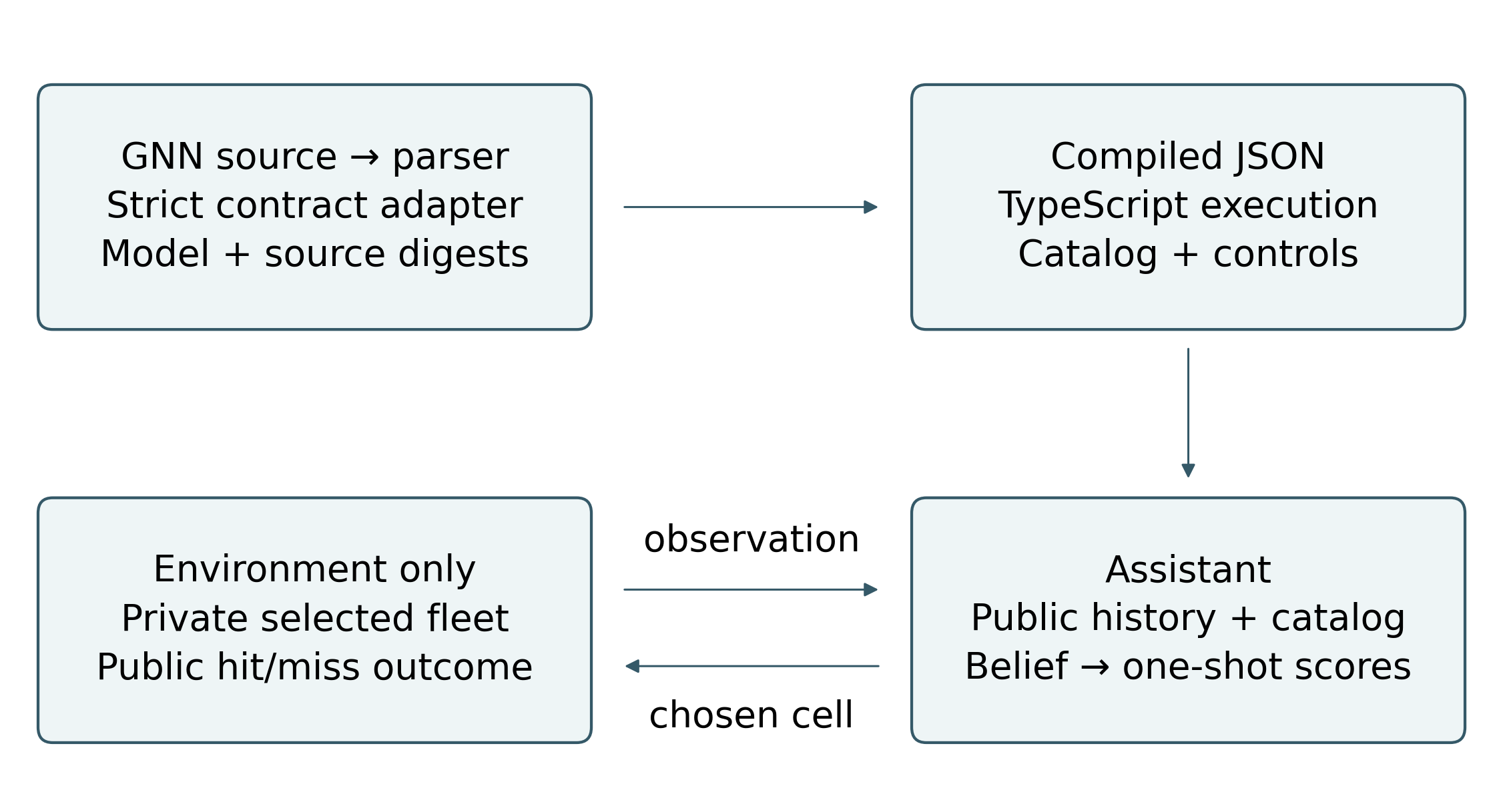
The Model & guide view follows the actual source-to-runtime path and downloads the verbatim GNN source and compiled JSON. A five-stage explanation separates declaration, upstream parsing, strict contract validation, compilation, and numerical execution. Runtime control overrides and catalog counts are recorded separately from the immutable specification defaults and digest. The decision explorer adds a fixed-axis plot of predicted hit probability against expected information gain for every legal action; it shares the policy table’s values, marks the selected and leading cells with distinct shapes, and explicitly discloses overlapping points. Under the symmetric binary likelihood, information is a function of the forecast and noise, so the plot is an interpretation aid rather than independent performance evidence.
Separate modules own legal fleets and random streams, game transitions, Bayesian inference and action scores, hypothetical analysis, event-sourced sessions, worker lifecycle, and reusable interface components. This arrangement follows the scientific-software principle of small components with explicit interfaces (Wilson et al. 2014). The browser has four views: Play, Agent diagnostics, Decision explorer, and Model & guide. Shared boards, controls, charts, and tables connect the same quantities across views. Six maps separately show occupancy, hit forecast, information gain, preference cost, weighted EFE, and action probability, with explicit scales and directions.
A separate typed ESM package exposes the core without browser, worker, Bun, or Python runtime imports. Its bundled default model is the already checked GNN compilation; consumption does not execute arbitrary GNN or revalidate a remote source. Headless commands run the actual two-actor game to a resumable replay or analyze either actor’s public observations with explicit temporary control overrides. These competitive games are distinct from the single-fleet demonstration below. Analysis reports are also distinct from replay files: they preserve impossible log weights with an explicit negative-infinity string instead of JSON’s silent conversion to null, and reject unexpected nonfinite values. CLI analysis reports record their runtime/version. Version-one replays carry no producer metadata and recompute opponent actions; retain the producing runtime separately and compare reconstructed histories when moving between engines. Final floating-point bits and near-tied choices can differ between engines. Source/artifact receipts and real Node, Bun, TypeScript-consumer, and local-archive checks support reuse; they do not establish scientific efficacy. Version 0.5.0 is publicly distributed through the release and archive identified below.
The sandbox starts from live controls, recalculates subjective beliefs when noise changes, and commits only through an explicit Apply action without firing a shot. Beta and precision sweeps instead hold the posterior fixed. Analysis snapshots contain public history, settings, posterior weights, action scores, counterfactual branches, and model identity. They are distinct from resumable replay files. Replays bind the model hash and preserve ordered action-relevant controls for runtime-sensitive seeded reconstruction. Workers support cancellation, stale-result protection, explicit failures, and bounded timeouts. The selected fleets can be reconstructed from local seeds: this is not cryptographically private multiplayer software.
4 Study designs and statistical comparisons
4.1 An analytic check of preference and information
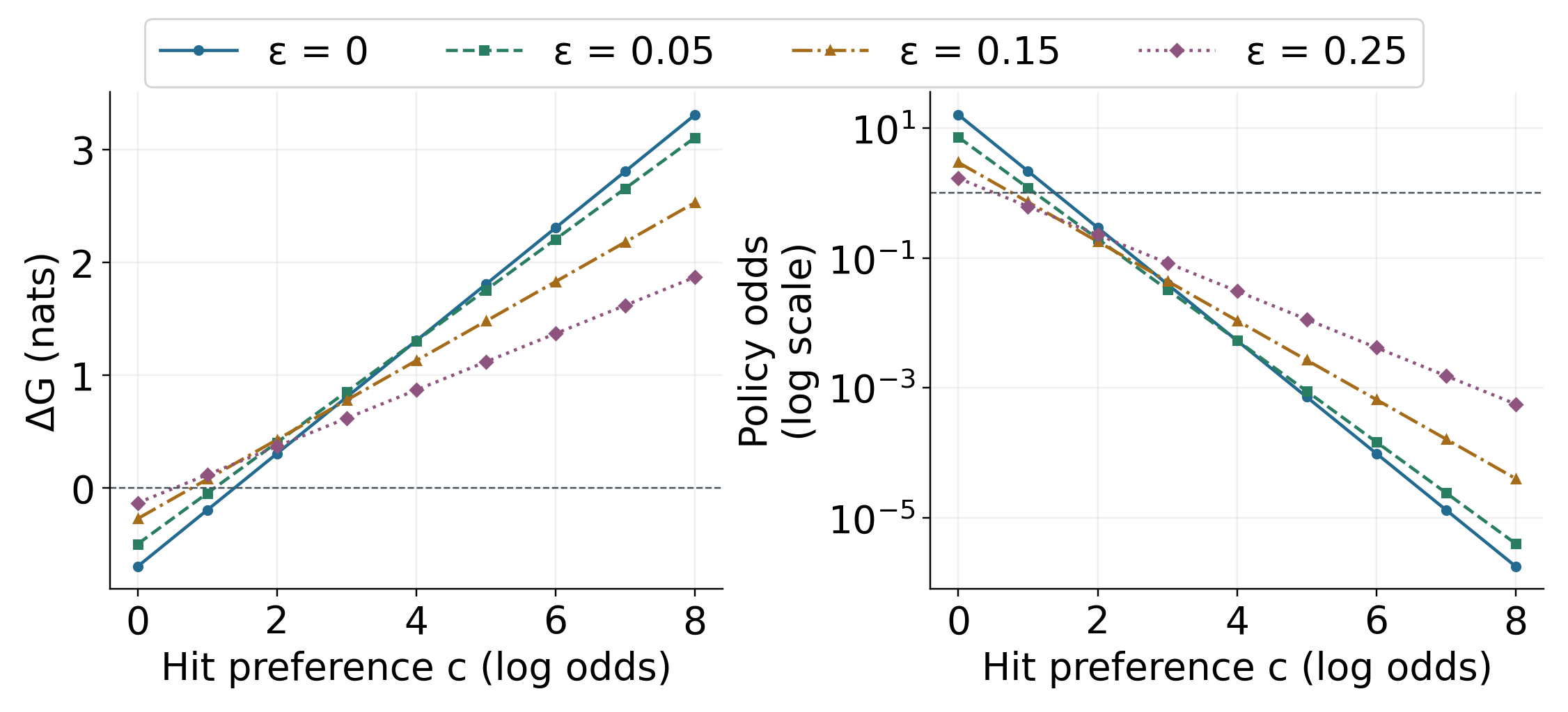
Example 1 (A guaranteed hit and a distinguishing observation). Consider two equally probable legal length-two fleets at cells \((0,1)\) and \((1,2)\) of a six-by-six board. Cell 1 is occupied under both hypotheses; cells 0 and 2 each distinguish them. For a common cell, \(p=1\), \(r=1-\epsilon\), and \(I=0\). For either distinguishing cell, \(p=1/2\), \(r=1/2\), and \(I=\log2-h(\epsilon)\). With uniform \(E\), the pairwise score difference is
\[G_\beta(\text{uncertain})-G_\beta(\text{common}) =(1/2-\epsilon)c-\beta[\log2-h(\epsilon)].\qquad{(10)}\]
In this example, for \(\beta=1\) and \(\epsilon=0\), the preference crossover is \(c=2\log2\). At \(c=1\) the distinguishing cell has lower score; at \(c=2\) the guaranteed hit has lower score. The pairwise policy odds are \(\exp[-\gamma\Delta G]\) even though other available cells share the policy’s denominator. The plot in fig. 2 shows this exact calculation from runtime scores. The example demonstrates an immediate trade-off, not fewer total shots: after the fleet is identified, its remaining occupied cells still need to be fired upon.
4.2 The exploratory sixteen case comparison
The finite benchmark asks how many distinct shots are needed to find all 17 occupied cells of one selected fleet. It excludes alternating turns, strategic placement, opponent behavior, and competitive win rates. Four strategies receive the same catalog and their own public outcomes: uniform random without replacement, greedy hit forecast, greedy information gain, and greedy minimum \(G_1\). The last is deterministic score selection, not sampling from the displayed \(q(a)\).
The protocol was written before the first result generation and fixes 16 seeds at each of two catalog sizes, 256 and 4096. Every seed–size case is run under all four policies, yielding 128 searches with no exclusions. Controls are \(\epsilon=0\), \(c=2\), \(\beta=1\), \(\gamma=4\), and \(k=0\). These deliberately differ from the browser’s startup defaults. Nonrandom scores break ties by higher predicted hit probability, then ascending cell index. Independent seeded streams construct the catalog, select the environment fleet, and choose random actions. The protocol records the exact offsets and seeds in machine-readable form.
Each policy selector receives only available action scores; an environment callback owns occupancy truth. Termination uses the public fleet segment count and observed hits. Every search must finish within the 100-cell board, with 17 hits and no repeated cell; failure aborts generation. Per-shot forecasts, expected information, posterior entropy, outcomes, catalog hashes, and source hashes are retained. Reporting is descriptive: all 16 cases, means, medians, ranges, and paired mean differences from greedy hit. No significance tests, tuned best-seed selection, or population confidence claims are made. The two catalog sizes alter both the prior support and the pool from which truth is selected, so differences between sizes are not an isolated computational scaling experiment.
4.3 A paired comparison of five search strategies
The known descriptive results motivated a separately specified follow-up; they are not retroactively converted into an inferential study. Before final searches, a private protocol, explicit case manifest, source hashes, runtime metadata, and dated pre-execution receipt fix 128 fresh catalog/truth units at each of 256 and 4096 labels. This is prospective specification, not public preregistration. SHA-256 derives separate 32-bit catalog, truth-selection, and random-policy seeds from master seed 20261025, with globally recorded collision rejection and exclusion of historical and pilot stream states. Each unit constructs a fresh catalog and selects one label uniformly; all five profiles share that unit’s catalog and truth. Independence is an assumption about the separately derived pseudorandom streams. The inferential target is this frozen generator and label-selection distribution within each size, not unrestricted Battleship. The strata are analyzed separately because changing size also changes support and the truth pool.
In the manuscript and figures, \(M\) consistently denotes catalog-label count, \(N\) remains board width, and \(n=128\) denotes paired units per stratum. The retained machine-readable protocol and seed-derivation description use N as a local catalog-size placeholder; that metadata spelling is preserved without changing any seeds or model dimensions.
4.3.1 Shared cases and declared selectors
The profiles are uniform random without replacement; pragmatic maximization of predicted hit probability; epistemic maximization of expected information gain; combined minimization of standard one-step \(G_1\); and minimization of information-weighted \(G_4\). The last is an explicit generalized objective, not standard EFE. All use \(c=2\), \(\epsilon=0\), uniform habits, and displayed precision \(\gamma=4\); precision does not affect these greedy choices. A new, prospectively fixed global absolute score band of \(10^{-12}\) is followed by the same band around maximum predicted hit and then ascending cell index. It avoids a nontransitive approximate sort and is distinct from the historical exact floating-point tie rule. No profile receives selected truth; only the environment callback returns outcomes.
The primary endpoint is completion shots \(T\), the shot receiving hit 17. Secondary endpoints are cumulative hits \(K_5\) after five shots and normalized catalog-label entropy \(H_5/\log M\). Lower favors a profile for completion and entropy; higher favors it for hits. Entropy counts label multiplicity, not distinct physical layouts. A zero-noise, uniform-label specialization filters surviving hypotheses using public observations and reuses the unchanged action scorer. Predetermined excluded pilots at both target sizes must agree with unchanged full-history inference within \(10^{-12}\) for occupancy, entropy, forecasts, information, and scores, with exactly matching selected cells. Deliberate numerical perturbations must fail. Complete legal traces, catalog hashes, selected-label identities, and time-zero conditions are retained. All 128 units per size and all five profiles are mandatory; failure aborts, with no exclusions, seed replacement, or optional stopping.
4.3.2 Endpoints and paired statistical analysis
For each non-pragmatic profile, size, and endpoint, the raw difference is profile minus pragmatic within a unit. The 24 planned comparisons form one step-down Holm family at \(\alpha=.05\) (Holm 1979). Familywise control relies on valid component p values under the stated paired-unit sampling assumptions; it does not require independence among the 24 tests. The word sequential in Holm’s procedure concerns ordered hypothesis rejections, not adaptive data collection. Exact two-sided paired sign tests test whether positive and negative differences are equally likely conditional on being non-tied; they do not test equality of means. The paired sign statistic uses directions rather than magnitudes (Dixon and Mood 1946). We condition on non-tied differences, as in the NIST technical reference; Dixon and Mood’s historical treatment instead split ties between the signs. Integer ties are exact; normalized-entropy differences within \(10^{-10}\) are sign-test ties. All-tie rows receive \(p=1\) by convention. The binomial test implementation and Holm procedure are identified explicitly. Favorable/tied/unfavorable counts always sum to 128 and refer to endpoint differences, not competitive wins.
Separately, 10,000 paired-unit bootstrap resamples give descriptive 95% percentile intervals for mean raw differences (Efron 1979, 1987). Each draw resamples a whole catalog/truth unit with its paired outcomes, rather than resampling the two profiles independently. Empirical bootstrap quantiles are an approximate interval method; we do not use bias-corrected and accelerated intervals or claim their higher-order properties. Ties and tiny raw entropy differences remain in those calculations. These approximate intervals are not simultaneous, do not guarantee finite-sample coverage, and are not inversions of the sign tests; excluding zero is not the Holm decision. Fixed per-comparison bootstrap seeds and the percentile method are recorded. Curves summarize all 128 units at each shot through 30, without inferential bands or curve-wise tests. Completed cases retain 17 hits and their actual terminal label entropy, which can remain positive for duplicate layouts. The complete protocol and all 24 comparisons accompany the manuscript.
5 Strategy performance across three search objectives
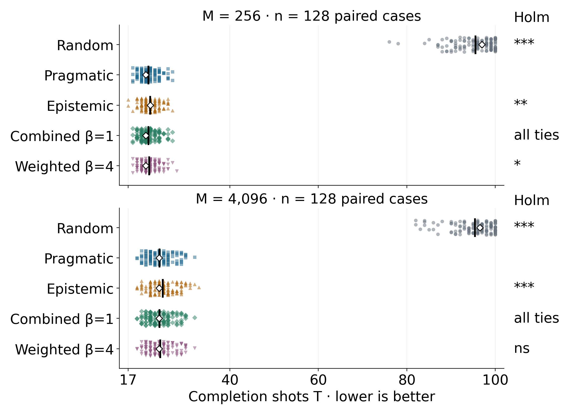
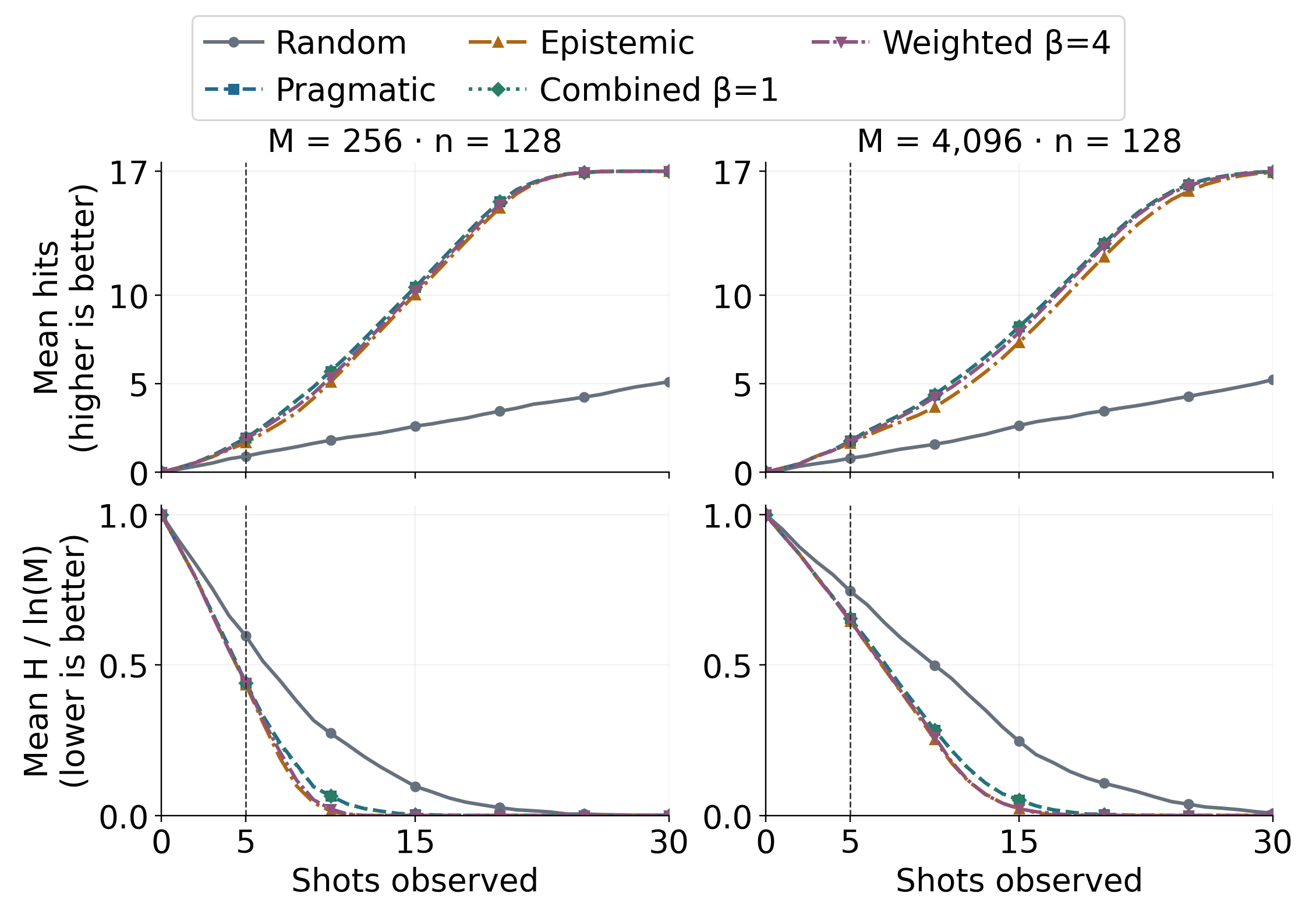
The prospectively specified follow-up completed all 1,280 searches (256 paired catalog/truth units, five profiles) in 47,975 shots, with no exclusions. Every summary below uses all 128 units within its catalog-size stratum. The original descriptive study is retained separately below.
| M | Profile | Mean completion shots | Mean hits at 5 | Mean label entropy at 5 |
|---|---|---|---|---|
| 256 | Random | 95.492 | 0.914 | 0.5965 |
| 256 | Pragmatic | 21.555 | 1.945 | 0.4407 |
| 256 | Epistemic | 21.953 | 1.688 | 0.4348 |
| 256 | Combined β=1 | 21.555 | 1.945 | 0.4403 |
| 256 | Weighted β=4 | 21.734 | 1.883 | 0.4407 |
| 4,096 | Random | 95.352 | 0.797 | 0.7455 |
| 4,096 | Pragmatic | 24.078 | 1.773 | 0.6547 |
| 4,096 | Epistemic | 24.797 | 1.664 | 0.6460 |
| 4,096 | Combined β=1 | 24.078 | 1.773 | 0.6547 |
| 4,096 | Weighted β=4 | 24.211 | 1.711 | 0.6475 |
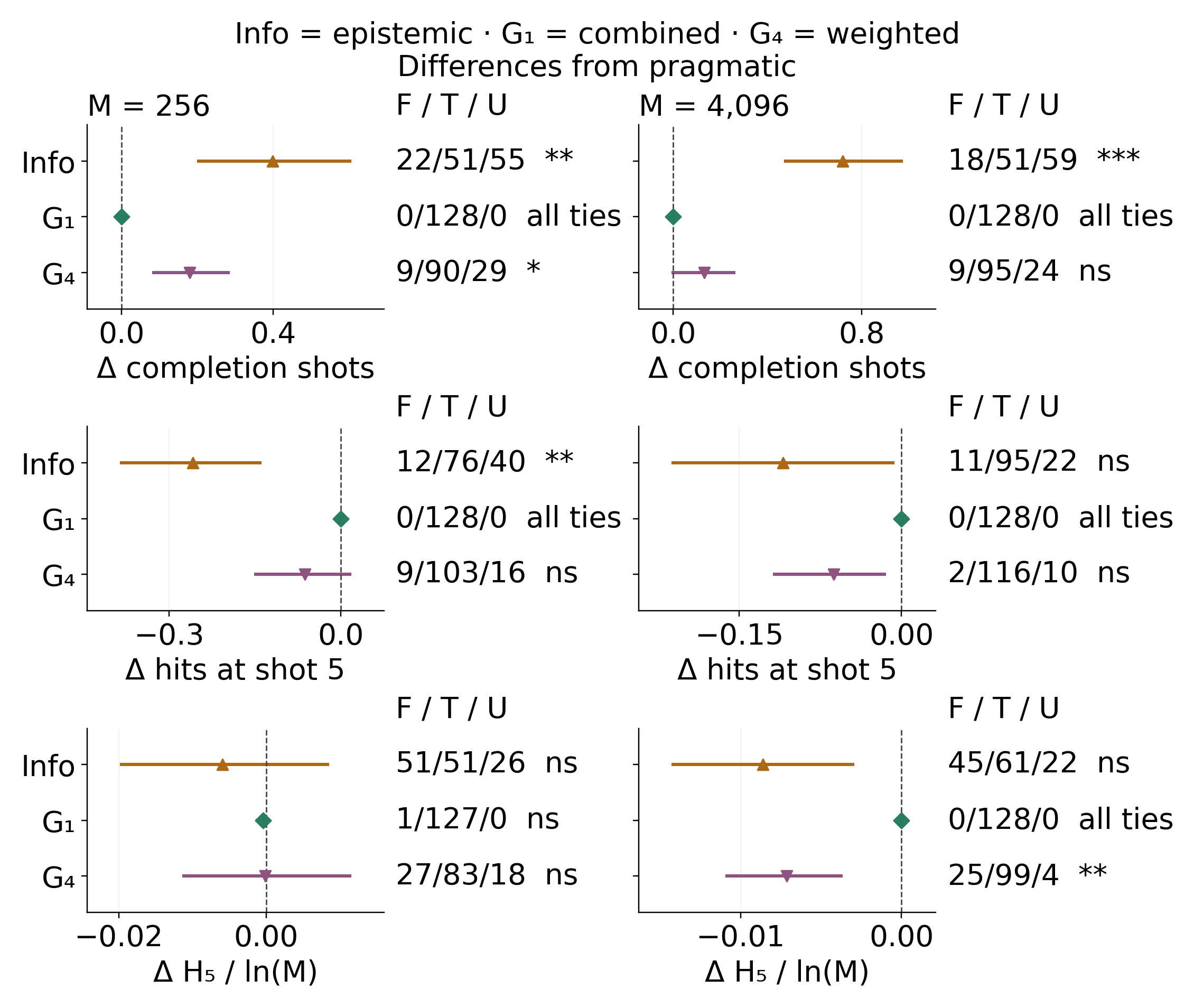
Pragmatic and combined profiles have equal completion counts in all 256 pairs. Epistemic completion is less favorable than pragmatic in 55 versus 22 non-tied cases at M = 256 and 59 versus 18 at M = 4096 (51 ties each); Holm-adjusted sign-test p values are 0.00325 and 0.0000580. Their paired mean excesses are 0.398 and 0.719 shots. Random requires more completion shots in every pair. These are conditional sign-balance rejections for this generator, not tests of equal means or unrestricted optimal play.
The information-weighted profile illustrates the distinction between identifying labels and completing a fleet. At M = 4096 its five-shot normalized entropy is lower than pragmatic in 25 cases, tied in 99, and higher in four (adjusted p = 0.00176); the mean difference is −0.00713. Its completion comparison is not rejected (adjusted p = 0.149). At M = 256 it instead has less favorable completion sign balance (adjusted p = 0.0232). No profile dominates every endpoint and stratum. Default EFE completion equality and non-rejection must not be described as proof of general equivalence.
5.1 All planned comparisons and their uncertainty
All differences are profile minus pragmatic. Favorable/tied/unfavorable counts have denominator 128, not the number of non-tied cases. Significance tests condition on non-ties; intervals estimate mean raw differences descriptively. Decimal rounding is for display only; decisions use full-precision adjusted p values. The complete protocol, seeds, traces, and analysis retain exact values.
5.1.1 Completion shots
| M | Profile | Mean Δ (95% interval) | F / T / U | Holm p |
|---|---|---|---|---|
| 256 | Random | +73.938 (+73.039, +74.773) | 0/0/128 | 1.41e-37 |
| 256 | Epistemic | +0.398 (+0.203, +0.602) | 22/51/55 | 0.00325 |
| 256 | Combined β=1 | +0.000 (+0.000, +0.000) | 0/128/0 | 1 |
| 256 | Weighted β=4 | +0.180 (+0.086, +0.281) | 9/90/29 | 0.0232 |
| 4,096 | Random | +71.273 (+70.352, +72.148) | 0/0/128 | 1.41e-37 |
| 4,096 | Epistemic | +0.719 (+0.477, +0.969) | 18/51/59 | 5.8e-05 |
| 4,096 | Combined β=1 | +0.000 (+0.000, +0.000) | 0/128/0 | 1 |
| 4,096 | Weighted β=4 | +0.133 (+0.000, +0.258) | 9/95/24 | 0.149 |
5.1.2 Hits after five shots
| M | Profile | Mean Δ (95% interval) | F / T / U | Holm p |
|---|---|---|---|---|
| 256 | Random | -1.031 (-1.297, -0.766) | 21/30/77 | 2.4e-07 |
| 256 | Epistemic | -0.258 (-0.383, -0.141) | 12/76/40 | 0.00204 |
| 256 | Combined β=1 | +0.000 (+0.000, +0.000) | 0/128/0 | 1 |
| 256 | Weighted β=4 | -0.062 (-0.148, +0.016) | 9/103/16 | 1 |
| 4,096 | Random | -0.977 (-1.273, -0.695) | 31/19/78 | 0.000139 |
| 4,096 | Epistemic | -0.109 (-0.211, -0.008) | 11/95/22 | 0.721 |
| 4,096 | Combined β=1 | +0.000 (+0.000, +0.000) | 0/128/0 | 1 |
| 4,096 | Weighted β=4 | -0.062 (-0.117, -0.016) | 2/116/10 | 0.386 |
5.1.3 Normalized label entropy after five shots
| M | Profile | Mean Δ (95% interval) | F / T / U | Holm p |
|---|---|---|---|---|
| 256 | Random | +0.1557 (+0.1096, +0.2001) | 33/0/95 | 8e-07 |
| 256 | Epistemic | -0.0059 (-0.0196, +0.0084) | 51/51/26 | 0.0763 |
| 256 | Combined β=1 | -0.0004 (-0.0012, +0.0000) | 1/127/0 | 1 |
| 256 | Weighted β=4 | -0.0001 (-0.0111, +0.0114) | 27/83/18 | 1 |
| 4,096 | Random | +0.0908 (+0.0558, +0.1244) | 34/0/94 | 2.17e-06 |
| 4,096 | Epistemic | -0.0086 (-0.0142, -0.0030) | 45/61/22 | 0.0809 |
| 4,096 | Combined β=1 | +0.0000 (+0.0000, +0.0000) | 0/128/0 | 1 |
| 4,096 | Weighted β=4 | -0.0071 (-0.0108, -0.0038) | 25/99/4 | 0.00176 |
5.2 The original exploratory comparison
The original 16 fixed cases per size used four profiles and exact floating-point tie ordering. Their 128 searches, source bindings, protocol, and unaltered figure formats remain in the source distribution. The table below is preserved; no retrospective p values or inferential intervals are assigned to those exploratory cases.
| Catalog | Policy | Mean shots | Median | Range | Mean Δ vs hit |
|---|---|---|---|---|---|
| 256 | Uniform random | 94.94 | 98.5 | 74–100 | +73.44 |
| 256 | Greedy hit | 21.50 | 21.5 | 18–25 | +0.00 |
| 256 | Greedy information | 21.56 | 21 | 18–26 | +0.06 |
| 256 | One-step EFE | 21.50 | 21.5 | 18–25 | +0.00 |
| 4,096 | Uniform random | 94.62 | 96 | 83–100 | +70.31 |
| 4,096 | Greedy hit | 24.31 | 24 | 20–30 | +0.00 |
| 4,096 | Greedy information | 25.12 | 25 | 22–32 | +0.81 |
| 4,096 | One-step EFE | 24.31 | 24 | 20–30 | +0.00 |
6 What the strategy comparisons establish
The follow-up separates endpoint goals instead of forcing a single strategy ranking. Pragmatic and combined completion counts tie in all 256 fresh pairs, while pure epistemic selection has less favorable completion sign balance in both size strata. At 4096 labels, the information-weighted profile more often reduces five-shot label entropy than pragmatic selection, but its completion comparison is not rejected. Learning which labels remain and taking predictable hits are different objectives. The figures retain their separate metrics and complete comparisons. Neither non-rejection nor all-tie observations establish general equivalence, and sign tests do not test equal means.
The original descriptive comparison remains separate: EFE and greedy-hit completion counts tied in all 32 pairs and ordered shot traces in 27. Greedy information required 0.0625 and 0.8125 more shots on average in its two strata. Those exploratory results informed the deliberate β = 4 contrast and five-shot endpoints. The privately frozen follow-up is not publicly preregistered. Neither study implies that information seeking is generally harmful or pragmatic search is optimal.
6.1 Why the objectives can select different shots
Under the zero-noise benchmark likelihood, information gain is binary entropy of the occupancy forecast. With uniform habits, minimizing the weighted score is equivalent to maximizing \(2p+\beta h(p)\) at the declared preference \(c=2\). Pure pragmatic choice instead maximizes \(p\), and pure epistemic choice maximizes \(h(p)\). Their continuous preferred probabilities are one and one half. For positive \(\beta\), the stationary point of the weighted value is \(p^*=(1+e^{-2/\beta})^{-1}\): about 0.8808 for combined \(\beta=1\) and 0.6225 for weighted \(\beta=4\). The derivative changes from positive to negative there. These values describe the objectives rather than fitting the observed search results. A particular finite board need not offer an action with that forecast.
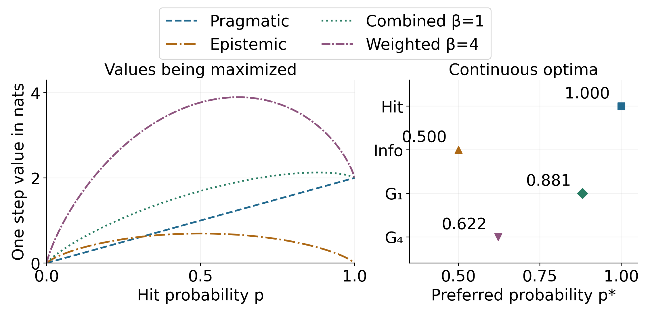
Equality of completion counts on the benchmark is an observed property of these cases, not a theorem that the scores rank actions identically. The two-fleet example demonstrates a disagreement at other controls. A small latent catalog can collapse after a few observations, after which posterior-based policies can target remaining known occupied cells. Random selection intentionally ignores that information. Its large completion counts should not be presented as a demanding comparison with state-of-the-art planners.
6.2 Inference support and external validity
The most important limitation is the inference space. The true label is sampled from the very catalog provided to the assistant. This in-distribution construction protects zero-noise inference from inconsistent observations, but makes no claim of robustness to an unseen fleet. The placement procedure is biased, and duplicate labels preserve multiplicity. Larger or differently sampled catalogs, out-of-support truths, alternative legal rules, and model uncertainty would require separate experiments. The present support is neither an exhaustive physical fleet space nor a learned approximation with quantified external error.
6.3 Planning horizon and feedback assumptions
Planning is also restricted. Re-evaluating a one-shot score after each observation does not evaluate future contingent shot sequences. Pure information gain concerns discrimination among hypotheses; completing a fleet search concerns a different task utility (Garnett et al. 2012). A multi-step reward-based planner can exploit information instrumentally (Kaelbling et al. 1998; Silver and Veness 2010). Appropriate future comparisons would share rules, priors, information access, budgets, and objectives, and would separate computation time from decision quality. They should include held-out fleet generation rather than assume that catalog-conditional accuracy transfers to unrestricted play.
Positive assumed noise is a transparent sensitivity control, not an estimated physical mechanism. Since actual feedback is truthful, Brier losses and surprise at positive noise diagnose the declared subjective model under mismatch. They do not establish calibration of a real sensor. Similarly, the spatial policy prior is manually specified, not learned, and the catalog posterior contains no neural dynamics or Dirichlet parameter updates. The active-inference interpretation is a finite mathematical specialization, without a claim of biological realism.
6.4 Educational use and specification limits
The interface offers plausible routes for teaching model inspection: a learner can distinguish occupancy from forecast, compare branch outcomes, verify an entropy identity, and change one setting without firing. No learner study, usability study, or clinical experiment has been performed. Existing tutorials and implementations already make active inference accessible (Smith et al. 2022; Heins et al. 2022); the dashboard’s educational value remains a hypothesis. Likewise, an executable GNN adapter establishes traceable model semantics for this backend, not validation of all upstream GNN transformations or proof that a specification is scientifically adequate.
7 Reproducing the software and manuscript
The source distribution retains both protocols, explicit fresh-case seeds, complete search traces, all planned comparisons, source and runtime bindings, analytic samples, figure-generation code, manuscript, and 34 references: 32 scholarly papers, a pinned software source, and a manufacturer manual. The original 21-entry dossier records selected substantive passages from 19 scholarly works, qualified manuscript reading alongside publisher-abstract evidence for one work, and the software source. The Battleship supplement adds selected substantive passages from seven scholarly papers and the manufacturer instructions. Several papers reuse tasks or question corpora; these are not seven independent replications. The statistical and search supplement adds five primary works on paired signs, step-down multiplicity, bootstrap inference, and post-hit Battleship decision trees. Its selected Holm and Efron 1987 readings use OCR transcriptions checked against publication metadata; clean publisher full text was unavailable for those readings. Together the dossiers record reading locations, DOI checks, task differences, and bibliographic ambiguities, without claiming systematic review or full-paper proof audits. The unread Lindley candidate and unresolved corrigendum remain excluded from stronger claims. The GNN concept DOI does not uniquely identify its pinned source bytes.
The build imports PDF, HTML, and DOCX renderers from the local
docxology/template repository. It records the imported
template-source hashes and output digests, while keeping authored
manuscript sources separate from generated products. The template
remains an independently versioned dependency. Seeds, versions, and
checksums help reconstruct a computation, but do not substitute for
data, environment details, meaningful tests, or rendered inspection
(Sandve et al.
2013; Wilson
et al. 2014). Machine-readable provenance follows relevant
Findable, Accessible, Interoperable, and Reusable (FAIR) principles
without asserting formal certification (Wilkinson et al.
2016).
Verification is layered. Numerical tests exercise Bayesian updates, expected and realized information, score identities, counterfactual branches, and tiny positive likelihoods. Contract checks use the actual upstream parser and reject unsupported semantics. Research tests check analytic action changes, deterministic ties, seeded reconstruction, legal unique shots, and explicit failures. Invalid-evidence and exhausted-search inputs are required to fail. Manuscript validation separately checks source freshness, complete case coverage, numerical table agreement, resolved references, figure presence, and rendered pages. The acceptance documentation records which checks were freshly run and which historical dashboard receipts remain source-continuous.
Reproducibility supports examination; it does not establish the truth or generality of an interpretation (Peng 2011). Numerical correctness, browser operation, document rendering, empirical efficacy, and publication approval remain separate claims. This manuscript reports software and a bounded computational demonstration. Version 0.5.0 makes the source, manuscript, and reproducibility materials publicly available; publication does not add an empirical efficacy claim.
7.1 GitHub release and Zenodo archive
The Active Inference Institute publishes source and reproducibility materials at the Institute’s public Battleship repository, with the exact version identified by the v0.5.0 release. The manuscript is archived on Zenodo, DOI 10.5281/zenodo.23676081. The same DOI appears on the PDF cover, in the abstract, and in the repository citation metadata. GitHub links to the Zenodo record; the record links back to the versioned repository release.
The archive distributes the PDF together with Word and HTML editions, a browser dashboard, a built core package, and source/research companions. The record DOI identifies this manuscript and its deposited companions; no separate software DOI or package-registry publication is claimed. The Git tag identifies the source version, while release checksums identify each downloadable artifact. Historical verification reports retain their original scope and dates; publication does not convert bounded numerical or browser checks into scientific efficacy evidence.
Authored prose uses American English. Stable GNN, replay, and API identifiers retain their original spelling for compatibility, as do published reference titles and frozen historical review records.
8 Conclusions and next experiments
A finite Battleship model can make active-sensing assumptions unusually concrete: hypotheses occupy cells, observations alter explicit weights, and an action’s preference and information terms can be inspected side by side. The GNN-based implementation turns that connection into composable software and reproducible records. Its most useful result is the ability to explain precisely what an assistant knows, what its objective values, and where those explanations stop. The analytic disagreement, observed completion ties, and distinct early-uncertainty results illustrate why inspectable objectives and paired endpoint comparisons are more informative than a blanket claim that an information-seeking strategy wins.
Next experiments should use held-out fleet generators and compare contingent planning under matched observations and computation budgets. A separate learner study is needed before making claims about educational benefit.
Version 0.5.0 is the organization and visual-explanation edition. The existing repository was transferred to the ActiveInferenceInstitute organization, retaining its history and prior release. Current metadata and the Pages site use the organization address; the initial manuscript deposit remains available under its original DOI. A narrated 20-minute lecture, captioned video, slides, transcript, and source ledger accompany this version’s release. The additional diagrams and motion explain retained quantities and software boundaries; they do not add experimental cases or renew scientific efficacy claims.